Mathematical Modeling of Dynamic Feedback Loops in Carbon Cycle Using Differential Equations

Francis Omondi Owino; Beatrice Adhiambo Odero Obiero; Vincent Bulinda

doi:doi:10.11648/j.mma.20261103.11

Research Article |

| Peer-Reviewed

Mathematical Modeling of Dynamic Feedback Loops in Carbon Cycle Using Differential Equations

Francis Omondi Owino^*

, Beatrice Adhiambo Odero Obiero, Vincent Bulinda

Published in Mathematical Modelling and Applications (Volume 11, Issue 3)

Received: 20 July 2026 Accepted: 7 August 2026 Published: 24 September 2026

Views: Downloads:

Download PDF

Share This Article

Twitter
Linked In
Facebook

Abstract

Carbon dioxide is very important during photosynthesis. However, it increases as a result of deforestation, burning of fossil fuels, cement manufacturing factories and other agricultural practices and this causes global warming. Carbon cycle as a process involves interactions among major reservoirs controlled by complex feed back relationships that are not easy to understand without a well organized mathematical framework. Some of the existing carbon cycle models are too complex while others are too simple and fail to include nonlinear feedback loops between reservoirs. This study built a model that captures the dynamic feedback interactions between the most relevant carbon reservoirs and investigate their effects on carbon partitioning and stability of the system through centuries. Carbon exchanges (sequestration, respiration, decomposition and interaction with the atmosphere) were simulated using a mathematical modeling approach based on systems of differential equations. Equilibrium and stability characteristics of the model were analyzed and the behavior of the model was examined numerically under various environmental conditions. These results demonstrated that feedback interactions are important for the regulation of carbon and in determining long-term equilibrium states. The model demonstrated that a disturbance in one of the reservoirs affects the entire system, changing the overall carbon dynamics. Conditions were identified under which the system stays in balance or changes to new states. The stability analysis showed conditions for maintaining a balance or changing to new state of the system. The study concluded that differential equation modeling provides a clear framework for understanding dynamic feedback loops in the carbon cycle. It is recommended that the model be extended to incorporate additional environmental variables and be used as a basis for further quantitative studies in climate and environmental modeling.

Published in	Mathematical Modelling and Applications (Volume 11, Issue 3)
DOI	10.11648/j.mma.20261103.11
Page(s)	53-69
Creative Commons	This is an Open Access article, distributed under the terms of the Creative Commons Attribution 4.0 International License (http://creativecommons.org/licenses/by/4.0/), which permits unrestricted use, distribution and reproduction in any medium or format, provided the original work is properly cited.
Copyright	Copyright © The Author(s), 2026. Published by Science Publishing Group

Keywords

Global Warming, Carbon Cycle, Reservoirs, Feedback Loops, Sequestration, Differential Equations, Eigenvalues, Eigenvectors

1. Introduction

The Global Carbon Cycle controls the movement of carbon between its reservoirs and ensures stability of Earth's climate

[1]

. Carbon fluxes are unbalanced by anthropological activities such as burning of fossil fuels, deforestation, and change in land use, which has resulted in the acceleration of climate change and increased amounts of carbon dioxide in the atmosphere

[2, 4]

. To predict the response of climates and to formulate mitigation policies, therefore, understanding climate dynamics and the behavior of the carbon cycle is crucial. Carbon cycle dynamics are regulated by positive and negative feed backs which control carbon fluxes between the Earth's major pools

[5, 6]

. Systematic analysis of these processes is made difficult by their interconnections at the nonlinear level, where mathematical models have to be applied

[7]

. Numerical models of carbon transfers, stability analysis of the system, and prediction of the system's long-term behavior are given by Ordinary Differential Equation (ODE) models

[8, 9]

. While the use of compartment- and process-based models has enhanced understanding of carbon cycles

[10]

, they lack an integration of many important feedback interactions and generally produce simplified estimates of carbon flux, which can result in limitations in the ability to capture transient responses or the resilience of a system to changing environmental conditions

[5, 11]

. A combination of feedback loop theory with dynamical systems analysis provides a broader perspective for studying carbon cycle behavior using equilibrium analysis, stability analysis, and numerical analysis

[12, 15]

. This research built a mathematical carbon cycle model with feedback loops between different parts, such that the conjunction of the parts is modeled with a system of ordinary differential equations. This model is analyzed using both equilibrium and local stability analysis, and through numerical simulations, to describe the interactions among anthropological emissions and carbon sequestration

[13, 17]

. The model also gives a mathematical description of the carbon cycle and assesses the feedback mechanisms and their effect on the long-term behavior of climate. The findings provide insight into the role of nonlinear feed backs in regulating carbon dynamics and demonstrate the usefulness of mathematical modeling in understanding the response of the carbon cycle to anthropocentric disturbances. Furthermore, the model was formulated and a numerical investigation was carried out, which are supported by mathematical and computational techniques. Classical numerical methods gave a strict framework to approximate solution of a system of ordinary differential equations, if analytical solutions are not available

[3]

. Mathematical biology

[14]

provides systematic methods for modeling interactions between interacting components to build and analyse biological and environmental dynamical systems further enhances the theoretical underpinning of constructing and analyzing biological and environmental dynamical systems. In addition, numerical simulations ran on accurate and efficient adaptive ordinary differential equation (ODE) solvers that have been widely tested for nonlinear dynamical systems and environmental models

[16]

giving a high degree of confidence in their ability.

2. Identification and Characterization of Carbon-Cycle Feed backs

Three main interacting carbon reservoirs were identified–atmospheric-carbon A(t), terrestrial carbon S(t), and oceanic carbon O(t), from a synthesis of recent carbon cycle studies and global Carbon-budget assessments. They are connected by photosynthesis, respiration, decomposition and atmosphere–ocean gas exchange, mediated by carbon fluxes. The interactions serves as conceptual foundation for the formulating of nonlinear differential-equation model. Overall, there were two main types of feedback identified. The atmosphere– terrestrial interaction is a positive feedback. Temporarily more carbon may lead to more respiration and decomposition that in turn will increase the amount of carbon released to the atmosphere. The nonlinear term- u(2, a(x, y, t)) represents this interaction. This interaction is conveyed by the nonlinear term, u(2, a(x, y, t)).

µAS,(1)

where µ represents the feedback strength. In contrast, carbon sequestration in the atmosphere–ocean system and sequestration in terrestrial ecosystems are stabilizing feed backs related to removing carbon from the atmosphere. The other terms are the oceanic uptake:

θA,(2)

with the atmosphere-ocean transfer coefficient θ. Competing reinforcing and stabilizing processes where used to represent these interactions in the model. This system was analyzed using equilibrium conditions,

\frac{dA}{dt} = \frac{dS}{dt}

\frac{dO}{dt}

= 0(3)

For the analysis of stability, the local stability analysis of the Jacobian matrix was performed. Locally asymptotically stable equilibrium (LASE): If all of the eigenvalues have negative real parts.

Re(λi) < 0.(4)

The magnitude of the reinforcing feed back coefficient µ suggests itself as an important determining variable of system behavior according to the analysis performed. Weak feedback will lead to a bounded equilibrium, while strong feed back can cause the amplification of a linear response, oscillations and instability.

3. Model Structure

3.1. Model Development Procedure

The global carbon cycle was modeled as a dynamic system with feedback loops between atmospheric carbon, natural sinks, and human emissions. Carbon inputs from fossil fuels and land-use changes increase atmospheric levels, while natural sinks remove carbon, generating negative feed back. The model focused on three key variables: Atmospheric Carbon C(t), Natural Sequestration (S(t), and Anthropological Emissions (E(t). The interactions between these variables form dynamic feedback loops where increased (C) stimulates (S), producing stabilizing negative feedback. Again, elevated(E) drives (C) upward, forming positive forcing. Finally (C) and (S) jointly influence (E) through policy or regulatory mechanisms, representing adaptive feedback. This framework is formalized mathematically by a system of coupled differential equations shown below:

\dot{C}

=−aC−bS+ fE,

\dot{S}

=cC−dS+kE, (5)

\dot{E}

=−lC−mS+nE,

In which a, b, c, d, f, k, l, m, n> 0 are positive constants and represent feedback strengths within the carbon cycle

Where:

a– Natural decay rate of atmospheric carbon (e.g., removal by oceans and land uptake).

b–Strength of negative feedback from sequestration on atmospheric carbon.

c–Enhancement of sequestration due to increased atmospheric carbon.

d–Natural decay rate of carbon in sequestration pools.

f–Contribution of anthropological emissions to atmospheric carbon growth

k–Effect of emissions on the sequestration pool.

l–Feed back of atmospheric carbon on emission growth(e.g., climate-induced emission changes).

m–Feed back of sequestration pools on emission dynamics.

n–Natural growth or decay of emissions (internal emission dynamics).

Also;

C: Excess atmospheric carbon concentration.

S: Excess carbon sequestration response.

E: Excess anthropological emissions.

The combined terms in system 5 above have the following physical interpretations:

1) aC: natural decay of atmospheric carbon,

2) bS: removal of carbon due to sequestration,

3) fE: contribution of emissions to atmospheric carbon,

4) cC: stimulation of sinks by increased carbon concentration,

5) dS: saturation or decay of sequestration capacity,

6) kE: degradation of sinks due to emissions and land-use change,

7) lC: emission reduction driven by climate pressure,

8) mS: dampening of emissions due to sink efficiency,

9) nE: growth-driven emission persistence.

Differentiating the first equation of system 5 with respect to time yields,

\frac{d^{2} C}{d t^{2}}

= -a

\frac{dC}{dt}

- b

\frac{dS}{dt}

+ f

\frac{dE}{dt}

(6)

From system 5, the time derivatives of S and E are given by;

\frac{dS}{dt}

= cC−dS+kE, (7)

And

\frac{dE}{dt}

= −lC−mS+nE (8)

Substituting equations (7) and (8) into equation (6) gives;

\frac{d^{2} C}{d t^{2}}

= −a

\frac{dC}{dt}

−b(cC−dS+kE)+ f(−lC−mS+nE), (9)

Expanding each bracket;

−b(cC−dS+kE) = - bcC + bdS - bkE (10)

And

f(−lC−mS+nE) = -flC - fmS + fnE (11)

Substituting equations (10) and (11) back into 9 we have,

\frac{d^{2} C}{d t^{2}}

= −a

\frac{dC}{dt}

- bcC + bdS - bkE -flC - fmS + fnE (12)

Collecting like terms in equation (12);

Carbon (C) terms = - bcC - flC = - (bc + fl)C (13)

Sequestration (S) terms = bdS - fmS = (bd - fm)S (14)

Emission (E) terms = fnE - bkE = (fn - bk) E (15)

Using these terms in equation (13), (14) and (15)

The equation (9) becomes,

\frac{d^{2} C}{d t^{2}}

= −a

\frac{dC}{dt}

- (bc + fl)C + (bd - fm)S + (fn - bk)E (16)

Moving all the terms to the left and equating to 0 we have;

\frac{d^{2} C}{d t^{2}}

\frac{dC}{dt}

+ (bc - fl)C - (fn - bk)E - (bd - fm)S = 0 (17)

Which is the same as;

\frac{d^{2} C}{d t^{2}}

\frac{dC}{dt}

+ (bc + fl)C + (bk - fn) E + (fm - bd)S = 0 (18)

From the first equation of system 5, expressing emission forcing term (E) in terms of C and S,

\frac{dC}{dt}

=−aC−bS+ fE,

Which is equivalent to;

−aC−bS+ fE =

\frac{dC}{dt}

(19)

fE =

\frac{dC}{dt}

+ aC + bS (20)

E =

\frac{\frac{dC}{dt} + aC + bS}{f}

(21)

E =

\frac{1}{f}

(

\frac{dC}{dt}

+ aC + bS) (22)

Substituting equation (22) into equation (18), we have;

\frac{d^{2} C}{d t^{2}}

\frac{dC}{dt}

+ (bc + fl)C +

(bk - fn)

[

\frac{1}{f}

(

\frac{dC}{dt}

+ aC + bS)] + (fm - bd)S = 0 (23)

The coefficient is

(bk - fn) \frac{1}{f}

(24)

Which is

\frac{(bk - fn)}{f}

(25)

Braking the bracket and multiplying throughout by coefficient equation (25)

\frac{d^{2} C}{d t^{2}}

\frac{dC}{dt}

+ (bc + fl)C +

\frac{(bk - fn)}{f}

(

\frac{dC}{dt}

+ aC + bS) + (fm - bd)S = 0(26)

Braking the bracket, we have;

\frac{d^{2} C}{d t^{2}}

\frac{dC}{dt}

+ (bc + fl)C +

\frac{(bk - fn)}{f} \frac{dC}{dt}

\frac{a(bk- fn)}{f}

C +

\frac{b(bk- fn)}{f}

S+ (fm - bd)S(27)

Combining the

\frac{dC}{dt}

terms, there are two first derivative terms in equation (27) above,

\frac{dC}{dt}

\frac{(bk - fn)}{f} \frac{dC}{dt}

(28)

Which is equal to;

(a +

\frac{bk - fn}{f}

)

\frac{dC}{dt}

(29)

(a +

\frac{bk}{f}

\frac{fn}{f}

)

\frac{dC}{dt}

(30)

(a +

\frac{bk}{f}

- n)

\frac{dC}{dt}

(31)

Combining the carbon terms, there are two carbon terms in equation (27) above,

(bc + fl)C +

\frac{a(bk- fn)}{f}

C (32)

Expanding

\frac{a(bk- fn)}{f}

We have

\frac{(bka- fna)}{f}

(33)

\frac{bka}{f}

\frac{fna}{f}

(34)

\frac{bka}{f}

- na (35)

Plugging this equation into equation (32) we have;

(bc + fl)C + (

\frac{bka}{f}

- na)C (36)

(bc + fl +

\frac{bka}{f}

- na)C (37)

Equivalent to;

\frac{bka}{f}

+ bc + fl - na (38)

Combining the sequestration terms from equation (27) above,

\frac{b(bk- fn)}{f}

S+ (fm - bd)S (39)

[

\frac{b(bk- fn)}{f}

+ (fm - bd)] S (40)

Making no any approximation at this stage; the

\frac{dC}{dt}

, carbon and sequestration terms i. e equations (32), (39) and (41), the equation (27) is reduced to;

\frac{d^{2} C}{d t^{2}}

+(a +

\frac{bk}{f}

- n)

\frac{dC}{dt}

+ (

\frac{bka}{f}

+ bc + fl - na)C + [

\frac{b(bk- fn)}{f}

+ (fm - bd)] S = 0 (41)

Using the slow sequestration approximation which implies that natural carbon sequestration evolves at a slower rate than atmospheric carbon;

S(t) ≈ 0,

Therefore we neglect the sequestration (S) terms, the equation (40) becomes;

\frac{d^{2} C}{d t^{2}}

\frac{bk}{f}

+ a - n)

\frac{dC}{dt}

+ (

\frac{bka}{f}

+ bc + fl - na)C= 0 (42)

This equation (42) is the equation of the model. It illustrates the dynamic response of atmospheric carbon under the combined effects of positive and negative feedback mechanisms.

Equation (42) is of the standard second-order linear differential equation form;

\frac{d^{2} C}{d t^{2}}

+ 2α

\frac{dC}{dt}

ω_{0}^{2} C

= 0, (43)

Where

α =

\frac{1}{2}

(

\frac{bk}{f}

+ a - n) (44)

And

ω_{0}^{2}

\frac{bka}{f}

+ bc + fl−na) (45)

The parameter

ω_{0}^{}

represents the natural response frequency of the carbon cycle system, while α measures the strength of damping due to stabilizing feed backs from natural sequestration and regulatory mechanisms. For

α^{2}

ω_{0}^{2}

, the system exhibits damped oscillatory behavior, indicating gradual recovery of atmospheric carbon concentration towards equilibrium following perturbations. Conversely, if

α^{2}

ω_{0}^{2}

, rapid divergence or overshoot occurs, suggesting potential instability within the carbon cycle. The entire three-variable feedback system in (5) reduces, after elimination of S(t) and E(t) under the slow–sequestration assumption, to a single governing equation for atmospheric carbon that has the structure of a damped feedback oscillator. The final single equation that summarizes the model is shown in equation (42) as,

\frac{d^{2} C}{d t^{2}}

+ (

\frac{bk}{f}

+ a - n)

\frac{dC}{dt}

\frac{bka}{f}

+ bc + fl−na)C =0

This single equation above is the final mathematical representation of the dynamic feedback carbon cycle model and compactly represents;

1) Positive forcing from emissions,

2) Negative stabilizing feed back from natural sequestration,

3) Regulatory feedback linking carbon levels to emissions,

4) The overall dynamic response of the carbon cycle as a damped second-order system.

Equivalently, this equation of the model can be express naturally in the form shown in equation (43), (44) and (45) respectively as:

\frac{d^{2} C}{d t^{2}}

+ 2α

\frac{dC}{dt}

ω_{0}^{2} C

= 0,

Where;

α =

\frac{1}{2}

(

\frac{bk}{f}

+ a - n)

And

ω_{0}^{2}

\frac{bka}{f}

+ bc + fl−na)

In the model framework, E acts as the primary forcing term, increasing C, while S represents the stabilizing feedback mechanism that removes part of the excess carbon from the atmosphere. The final model given in Equation (42) expressed as;

\frac{d^{2} C}{d t^{2}}

+ (

\frac{bk}{f}

+ a - n)

\frac{dC}{dt}

\frac{bka}{f}

+ bc + fl−na)C =0

is equivalent to zero as it represents the natural or intrinsic dynamics of the carbon cycle system after all interacting variables have been put into a single governing equation. In the derivation process, all terms containing the dependent variable C(t) and derivatives of it are moved to the left-hand side of the equation, while the forcing term of E(t) is put on the right-hand side of the equation. The evolution of the amount of carbon in the atmosphere is therefore solely dependent on the interaction and feedback inside the model by the model parameters. The zero on the right-hand side thus means that no additional external forcing (e.g., additional anthropological emissions, other time-varying inputs) are considered in the analysis of the system. If such external influences would have been taken into account, the equation would have been written as;

\frac{d^{2} C}{d t^{2}}

+ (

\frac{bk}{f}

+ a - n)

\frac{dC}{dt}

\frac{bka}{f}

+ bc + fl−na)C =F(t) (46)

Reduced carbon-cycle equation is a 2nd order linear ODE with constant coefficient. The form’s properties are noted as follows: It is second order because the highest derivative term is

\frac{d^{2} C}{d t^{2}}

and linear because the variables C(t) and its derivatives are not multiplied together nor evaluated inside of nonlinear functions in the form. In the absence of an external forcing function F(t), the equation becomes homogeneous, and describes the free response of the carbon-cycle system to the internal feedback mechanisms. Coefficients a, b, c, f, k, l, n have been taken as constants for the analysis. This equation is not linear in the independent variable (t) and is called autonomous. These properties enable the utilization of the characteristic equation for analytical solutions and exploring the stability and long term behavior of atmospheric carbon dynamics. If an external forcing term F(t) is added, the equation then becomes non-homogeneous, corresponding to the response of the system to carbon inputs or perturbations from outside the system.

3.2. Diagrammatic Representation of Dynamic Feed Back Loop Model

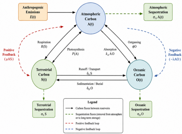
The dynamic feed back loops model developed in this study is illustrated in Figure 1. The diagram shows the interactions among atmospheric carbon concentration C(t), natural carbon sequestration S(t), and anthropological emissions E(t). Positive forcing arises from anthropological emissions that increase atmospheric carbon, while natural sequestration provides a stabilizing negative feedback by removing carbon from the atmosphere. In addition, atmospheric carbon and sequestration influence emission dynamics through regulatory and adaptive responses. These interacting feed back mechanisms collectively determine the dynamic behavior of carbon cycle and form the basis of the coupled differential equation system presented in Equation (5).

Download: Download full-size image

Figure 1. Dynamic feedback loop model.

The figure above shows Dynamic feedback loops model of the carbon cycle showing interactions among anthropological emissions, atmospheric carbon, and natural sequestration. Solid arrows represent carbon-flow interactions while dashed arrows represent regulatory feedback mechanisms.

3.3. Compact Mathematical Representation of the Carbon Cycle Feedback Model.

To present the developed model in a compact and rigorous mathematical structure suitable for analysis, the three coupled differential equations in (5) are expressed in vector–matrix form and subsequently reduced to a single governing equation for atmospheric carbon.

3.3.1. Vector–Matrix Form of the Full System

Let the state vector be defined as X(t)=

(\begin{matrix} \binom{C (t)}{S (t)} \\ E (t) \end{matrix})

(47)

Then the system in (5) i.e

\dot{C}

=−aC−bS+ fE,

\dot{S}

=cC−dS+kE,

\dot{E}

=−lC−mS+nE,

can be written compactly as;

\frac{dX}{dt}

= AX, (48)

where the system matrix is given by;

(\binom{_a _b f}{\begin{matrix} c_d k \\ _l_m n \end{matrix}})

(49)

The matrix equation (49) above represents the complete coupled carbon–sink–emission feedback system as a linear autonomous dynamical system.

3.3.2. Reduction to a Single Governing Equation

Differentiating the first equation of (5) with respect to time and substituting for

\dot{S}

and

\dot{E}

from the remaining equations yields the second–order equation (18) shown as;

\frac{d^{2} C}{d t^{2}}

\frac{dC}{dt}

+(bc+ fl)C+(bk− fn)E+(fm−bd)S = 0.

From the first equation of (5), the emission term is expressed as shown in equation (22)

\frac{1}{f} (\frac{dC}{dt}

+aC+bS)

Substituting the above expression into the second–order equation and invoking the slow–sequestration assumption (S ≈ 0), the system reduces to equation (42)

\frac{d^{2} C}{d t^{2}}

+ (

\frac{bk}{f}

+ a - n)

\frac{dC}{dt}

\frac{bka}{f}

+ bc + fl−na)C =0

3.3.3. Damped Oscillator Representation

The damped oscillator is represented by the reduced equation of the standard form of a second–order linear differential equations (43), (44) and (45) respectively as shown below;

\frac{d^{2} C}{d t^{2}}

+ 2α

\frac{dC}{dt}

ω_{0}^{2} C

= 0,

Where;

α =

\frac{1}{2}

(

\frac{bk}{f}

+ a - n)

And

ω_{0}^{2}

\frac{bka}{f}

+ bc + fl−na)

3.3.4. Final Mathematical Representation of the Model

The developed carbon cycle feedback model is therefore represented equivalently by the full coupled system 48 i.e

\frac{dX}{dt}

= AX,

and the reduced atmospheric carbon equation (43) i.e

\frac{d^{2} C}{d t^{2}}

+ 2α

\frac{dC}{dt}

ω_{0}^{2} C

= 0,

This compact formulation shows that the global carbon cycle, governed by interactions among atmospheric carbon, natural sequestration, and anthropological emissions, behaves dynamically as a damped second–order feedback system.

3.4. Numerical Verification of the Model

To examine the stability and dynamic behavior of the developed carbon cycle feed back model, representative secondary parameter values are chosen to reflect typical response rates within the Earth system. These values are chosen to illustrate the qualitative dynamics of the model rather than to fit specific empirical data sets. The system of ordinary differential equations was solved numerically using the classical fourth-order Runge–Kutta method (RK4). In MATLAB implementation, the results were computed using a fixed-step RK4 scheme and verified using the built-in solver ode45, which is based on an adaptive Runge–Kutta method.

3.4.1. Matrix Representation of the Carbon Cycle Model

System 5 can be written in matrix-vector form as:

\frac{d}{dt}

[\begin{matrix} C \\ S \\ E \end{matrix}]

[\begin{matrix} _a_b f \\ c_ d k \\ _l_m n \end{matrix}] [\begin{matrix} C \\ S \\ E \end{matrix}]

(50)

Letting X = [C S E]T, equation above becomes,

\dot{X}

=AX

where A is the system Jacobian matrix. The carbon cycle is asymptotically stable if all eigenvalues of matrix A have negative real parts, implying that there is perturbations in atmospheric carbon decay over time due to dominant negative feed backs from sequestration processes. Let the parameters from the above matrix form be:

a =1.8, b =3.2, c =0.25, d =0.9, f =1.1, k =0.18, l =2.0, m =0.85, n =0.45.

Substituting these values into system (50) yields:

\frac{d}{dt}

[\begin{matrix} C \\ S \\ E \end{matrix}]

[\begin{matrix} _1.8_3.2 1.1 \\ 0.25_ 0.9 0.18 \\ _2.0_0.85 0.45 \end{matrix}] [\begin{matrix} C \\ S \\ E \end{matrix}]

(51)

This system can be expressed compactly as;

\dot{X}

=AX (52)

where A denotes the Jacobian matrix of the carbon cycle feedback system.

3.4.2. Eigenvalues and Eigenvectors of Matrix A

Eigenvalues

The eigenvalues of matrix above are as shown below:

λ1 = −1.0885 +1.4880i

λ2 = −1.0885 −1.4880i

λ3 = −0.0730

Eigenvectors

Each eigenvector corresponds to its respective eigenvalue.

Eigenvector corresponding to λ1 = −1.0885 + 1.4880i

V_{1} = [\begin{matrix} 0.7101 \\ 0.0265 - 0.1875i \\ 0.5363 + 0.4151i \end{matrix}]

Eigenvector corresponding toλ2=−1.0885−1.4880i

V_{2} = [\begin{matrix} 0.7101 \\ 0.0265 + 0.1875i \\ 0.5363 - 0.4151i \end{matrix}]

Eigenvector corresponding toλ3=−0.0730

V_{3} = [\begin{matrix} 0.1433 \\ 0.2517 \\ 0.9571 \end{matrix}]

3.4.3. Eigenvalue Stability Analysis

The stability of equilibrium state is determined by solving the characteristic equation,

det(A−λI)=0. (53)

The resulting eigenvalues are as shown above, Since all eigenvalues possess negative real parts, the equilibrium of carbon cycle feedback system is asymptotically stable. The presence of a complex conjugate pair indicates oscillatory adjustment of atmospheric carbon concentrations due to delayed feed back mechanisms within the climate system. From the reduced second-order feedback equation (43) i.e;

\frac{d^{2} C}{d t^{2}}

+ 2α

\frac{dC}{dt}

ω_{0}^{2} C

= 0,

The damping coefficient α and natural frequency

ω_{0}

are given respectively as:

α =

\frac{1}{2}

(

\frac{bk}{f}

+ a - n)

And;

ω_{0}^{2}

\frac{bka}{f}

+ bc + fl−na)

Substituting the numerical values yields:

α=

\frac{1}{2}

(0.524+1.8−0.45)=0.937,

ω_{0}^{2}

=0.942+0.800+2.200−0.810=3.132,

hence,

ω_{0}

= 1.77

The corresponding recovery period is:

T_{0}

\frac{2 π}{ω_{0}}

= 3.55 time units

3.4.4. Stability Condition

Evaluating the stability criterion:

α^{2}

= 0.878 <

ω_{0}^{2}

= 3.132,

confirms that the system exhibits damped oscillatory convergence toward equilibrium.

3.5. Significance of the System Matrix, Eigenvalues, and Eigenvectors

3.5.1. Role of the Matrix A

In the carbon cycle model, the system is expressed as a set of linearized differential equations:

\frac{dC}{dt}

=AC+B (54)

Where;

1) C(t) is a vector representing carbon stocks in different reservoirs (e.g., atmosphere, oceans, biosphere),

2) A is a matrix representing the interactions and feedback among these reservoirs,

3) B represents external inputs, such as anthropological emissions.

Thus, the matrix A encodes how each carbon pool affects the others.

3.5.2. Significance of Eigenvalues

The eigenvalues of A describe the stability and dynamics of the system:

1) Real part of eigenvalues: If negative → the corresponding mode decays over time (stabilizing feed back). If positive → the mode grows over time (amplifying feedback).

2) Imaginary part of eigenvalues: If nonzero → the mode exhibits oscillatory behavior, i.e., carbon concentrations oscillate between pools

From the MATLAB output:

λ_{1,2}

= −1.0885 ± 1.4880i,

λ_{3}

= −0.0730 The negative real part of

λ_{1,2}

indicates that this mode decays, so the system tends toward stability. The imaginary part of

λ_{1,2}

implies oscillatory behavior, representing cyclic carbon fluxes between reservoirs before stabilizing. The small negative eigenvalue

λ_{3}

represents a slowly decaying mode, corresponding to long-term adjustments in reservoirs such as deep ocean or soil carbon

3.5.3. Significance of Eigenvectors

Eigenvectors describe the distribution of carbon among the reservoirs for each mode:

1) For

λ_{1}

and

λ_{2}

, eigenvectors show how the oscillations involve each reservoir. For example, a positive component in the atmosphere and negative in the ocean indicates carbon is moving from one pool to another.

2) For

λ_{3}

, the eigenvector indicates which reservoir is dominantly affected by the slow mode, typically a reservoir that adjusts most slowly (e.g., ocean or soil).

3.6. Selection of Parameters

The parameter values, i.e; a =1.8, b =3.2, c =0.25, d =0.9, f =1.1, k =0.18, l =2.0, m =0.85, n =0.45 were selected to satisfy mathematical consistency, stability requirements, and realistic feedback hierarchy within the linearized carbon feedback framework. All parameters values above, though not fitted to a specific data set are positive (0 < a, b, c, d, f, k, l, m, n), representing physical processes. Weak feedback or slow processes range from 0.01 to 0.5. Moderate or typical Earth system processes range from 0.5 to 2.5 while Strong feedback is greater than 2.5.

3.7. Graphical Illustration of the Model Dynamics

To further understand the behavior of carbon cycle model, graphical illustrations were used to visualize the temporal evolution of atmospheric carbon, the phase interaction between variables, and the influence of parameter variation on system stability. All simulations are based on a clearly defined numerical setup to ensure reproducibility and consistency of results.

3.7.1. Time Interval

All simulations are performed over the finite time horizon

t∈[0,20], (55)

with sufficiently fine resolution to accurately capture transient and oscillatory behavior.

3.7.2. Time Series Behavior of Atmospheric Carbon

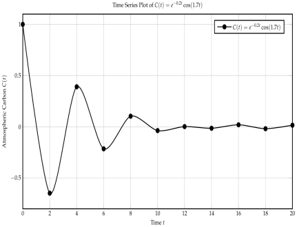
The time series illustrates the evolution of atmospheric carbon concentration C(t) over time. The solution is obtained from the first component of the numerical solution vector X(t).

The Table 1 above matches the exact analytical solution used in the graph below and it shows the decay term

e^{-0.2 t}

(damping effect).

The time series illustrates the evolution of atmospheric carbon concentration C(t) over time. The solution is obtained from the first component of the numerical solution vector X(t).

Table 1. Sample of numerical values used to generate the time series plot.

Time t	$e^{-0.2t}$	C(t)= $e^{-0.2t}$ cos(1.7t)
0	1.0000	1.0000
2	0.67032	-0.64806
4	0.44933	0.39065
6	0.30119	-0.21513
8	0.2019	0.10331
10	0.13534	-0.037239
12	0.090718	0.0018462
14	0.06081	-0.01434
16	0.040762	0.019416
18	0.027324	-0.018722
20	0.018316	0.015542

3.7.3. Time Series Graph

Download: Download full-size image

Figure 2. Atmospheric carbon concentration against time showing a damped oscillatory behavior due to the exponential decay term e−0.2t.

The time series results graph 1 directly confirm the stability properties obtained from the Jacobian and eigenvalue analysis. Since the system is governed by

\dot{X}

= AX, its behavior is determined by the eigenvalues of A. The presence of complex conjugate eigenvalues with negative real parts predicts damped oscillations. This is observed in the alternating but decreasing values of C(t), where the oscillatory sign changes reflect the imaginary components of the eigenvalues, while the gradual reduction in amplitude reflects the negative real parts. The exponential decay term in the numerical solution further confirms this stabilizing effect.

Thus, the graphical and tabulated results provide a direct numerical verification of the analytical result that the system is asymptotically stable, as all eigenvalues satisfy Re(

λ_{i}

) < 0, ensuring convergence towards equilibrium.

3.7.4. Phase Portrait of the Carbon System

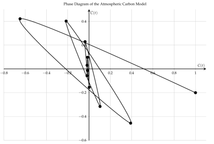
The phase diagram represents the relationship between atmospheric carbon concentration C(t) and its rate of change

\dot{C}

(t). Here,

\dot{C}

(t) is computed directly from the governing equation

\dot{C}

(t) = −aC−bS+ fE, using the numerically obtained trajectories of C(t), S(t), and E(t).

Below is a suitable table representing the numerical source of the plotted phase trajectory.

Table 2. Sample numerical values used to generate the phase diagram of the carbon system.

Time t	C(t) = $e^{-0.2 t}$ cos(1.7t),	$\dot{C}$ (t)
0	1.0000	0.20000
2	-0.64806	0.42081
4	0.39065	-0.45556
6	-0.21513	0.40138
8	0.10331	-31555
10	-0.037239	0.22864
12	0.0018462	-0.15456
14	-0.01434	0.097594
16	-0.019416	-0.057047
18	-0.018722	0.030088
20	-0.015542	-0.013365

3.7.5. Phase Diagram

The phase diagram is generated para-metrically from

C(t) =

e^{-0.2 t}

cos(1.7t),

\dot{C}

(t)= −0.2

e^{-0.2 t}

cos(1.7t) − 1.7

e^{-0.2 t}

sin(1.7t)

Download: Download full-size image

Figure 3. Phase trajectory of the carbon system showing a damped spiral approaching the equilibrium point at the origin.

The phase portrait shown in Table 2 and Figure 3 describes the relationship between C(t) and

\dot{C}

(t) for the carbon cycle model. The trajectory is generated from a damped oscillatory system, where both variables exhibit alternating signs while their magnitudes decrease over time. The plotted points show that the system starts from an initial state (1.0000,−0.2000) and progressively approaches values near the equilibrium (0,0) as (t) increases. This indicates that both atmospheric carbon concentration and its rate of change decay with time. Graphically, the phase diagram forms an inward spiral converging to the origin, reflecting oscillatory behavior with decreasing amplitude. This is caused by the interaction of periodic dynamics (sine and cosine terms) and exponential damping. In terms of system dynamics, this behavior confirms that the carbon cycle model is asymptotically stable. The spiral convergence is consistent with complex eigenvalues with negative real parts, which induce oscillations while ensuring eventual decay towards equilibrium.

4. Stability Behavior Under Parameter Change

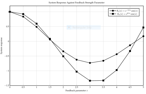
The Table 3 above matches the two functions plotted in the graph in Figure 4 below. It clearly shows decay in amplitude for the stable system and growth in size for the unstable system. The symmetric sign changes reflect oscillatory feedback effects.

Table 3. Sample numerical values illustrating system response under varying feedback strength parameter.

Feedback	cos(x)	Stable Rs(x)= Unstable Parameter x	( $e^{-0.1 x} cos (x)$ ) Ru(x)= $e^{-0.1 x}$
0.0	1.0000	1.0000	1.0000
0.5	0.87758	0.83478	0.92258
1.0	0.5403	0.48889	0.59713
1.5	0.070737	0.060884	0.082185
2.0	-0.41615	-0.34071	-0.50828
2.5	-0.80114	-0.62393	-1.0287
3.0	-0.98999	-0.7334	-1.3364
3.5	-0.93646	-0.65991	-1.3289
4.0	-0.65364	-0.43815	-0.97512
4.5	-0.2108	-0.13441	-0.33059
5.0	0.28366	-0.17205	0.46768

The symmetric sign changes reflect oscillatory feedback effects. The chosen step size (0.5) gives sufficient resolution for the presentation as shown in the graph below.

Download: Download full-size image

Figure 4. Comparison of stable and unstable system responses as the feedback strength parameter varies. The stable response decays while the unstable response grows in magnitude.

The bifurcation diagram shows how the stability of atmospheric carbon depends on feed back strength. A critical threshold separates stable and unstable regimes: below it, negative(stabilizing)feed back dominates and the system remains stable, while above it, positive feed back leads to instability and divergence. Thus, weak emission feed back maintains stability through sequestration effects, whereas stronger feed back causes a qualitative change in system behavior at the bifurcation point, leading to instability.

4.1. Interpretation of the Graphical Results

The graphical results collectively validate the analytical findings obtained from eigenvalue and stability analysis. The time series confirms damped oscillations in atmospheric carbon concentration, the phase portrait demonstrates inward spiral convergence toward equilibrium, and the bifurcation analysis shows how parameter variation can shift the system between stable and unstable regimes. Together, these results confirm that the carbon cycle model is dynamically stable under the chosen parameter configuration and that its behavior is strongly governed by feed back interactions between carbon reservoirs.

4.2. Simulation Setup for Graphical Results

Graphical analysis is used to illustrate the dynamic behavior, stability, and feed back interaction of atmospheric carbon concentration. The numerical simulations are carried out using the system;

\dot{X}

=AX

With the parameter set

a=1.8, b=3.2, c=0.25, d=0.9, f=1.1, k=0.18, l=2.0, m=0.85, n=0.45.

Initial Conditions: The system is initialized at a perturbed state away from equilibrium in order to observe its dynamic response:

X(0)=

(\begin{matrix} \binom{C(0)}{S(0)} \\ E(0) \end{matrix})

[\begin{matrix} 1.0 \\ 0.5 \\ 0.8 \end{matrix}]

(56)

5. Applications of the Developed Model

The resulting coupled nonlinear model involving differential equations was numerically by use of the classical fourth order Runge–Kutta (RK4) method to explore the carbon dynamics, equilibrium behavior, stability, parameter sensitivities, and emission scenarios.

It was shown by the numerical simulations that there is a dynamic exchange of carbon, that is, dynamic turnover of carbon, between the components of the carbon cycle: the atmosphere, the oceans and the terrestrial reservoirs. Rising anthropological emissions increased the carbon in the atmosphere, while the sequestration of the atmosphere in land and ocean worked as balancing processes. The results showed local asymptotic stability for the system with the baseline parameters. With the baseline parameters the system displayed damped oscillations that reached a stable equilibrium state. The equilibrium state was calculated by taking the average over time from

\frac{dCi}{dt}

= 0 i = 1,2,….n (57)

Feedback and sequestration coefficients were found to be highly sensitive to affect the atmospheric carbon dynamics (from sensitivity analysis). Oscillator strength, mean carbon levels, and the length of start up time were all enhanced by greater positive feedback, while greater sequestration rates helped speed up the convergence to the mean. Positive feedback and emissions strengthen the oscillations; the higher the strength of the positive feedback and the higher the amount of such emissions, the stronger the oscillation; mean carbon levels are also increased; greater sequestration rates shorten the start up period. Use of scenario analysis also showed that the intensity of feedback and anthropological emissions are the leading control on the carbon cycle's long-term behavior.

Overall, the model offers a mathematical tool for studying the interactions between carbon reservoirs, feed back, as well as the equilibria, stabilities and responses of the model to changes in carbon reservoirs and emission rates.

6. Results and Discussion

The study performed a stability analysis for the carbon-cycle feedback system. The behavior carbon-cycle feed back model was explored numerically using the linear system.

\frac{dX}{dt} = A

where the system matrix is A =

[\begin{matrix} _a_b f \\ c_d k \\ _l_m n \end{matrix}]

In the following, the values I used are for the parameter set; (a, b, c, d, f, k, l, m, n) = (1.8, 3.2, 0.25, 0.9, 1.1, 0.18, 2.0, 0.85, 0.45),

the matrix becomes A=

[\begin{matrix} _1.8_3.2 1.1 \\ 0.25_ 0.9 0.18 \\ _2.0_0.85 0.45 \end{matrix}]

6.1. Eigenvalue-Based Stability

The characteristic equation (53);

det(A−λI)=0.

gives the eigenvalues

λ2=−1.0885−1.4880i, λ3 = −0.0730.

Hence,

max_{i} {Re(λi)}

= −0.0730 < 0.

The pair of complex conjugates yields oscillatory modes, and the other half of the real parts of each are negative, leading to the damping of the modes over time. The third eigenvalue λ3 = −0.0730 is a slower decaying mode, and indicates the existence of different adjustment timescales in the system.

It was concluded that the general modal solution is;

X(t) =

c_{1} v_{1} e^{λ 1 t}

c_{2} v_{2} e^{λ 2 t}

c_{3} v_{3} e^{λ 3 t}

, (58)

Here

v_{i}

are the related eigenvectors. The complex eigenvalues introduce the terms of the form;

e^{-1.0885t} [A_{1}

cos(1.4880t)+

A_{2}

sin(1.4880t)], (59)

while the slow mode is portrayed as,

A_{3} e^{-0.0730t}

(60)

Thus the system is composed of an (exponentially) rapidly damped oscillatory part and a slowly decaying part.

6.2. Reduced-Order Atmospheric Carbon Dynamics

The following equation (12) models the reduction of atmospheric-carbon:

\frac{d^{2} C}{d t^{2}}

+ (

\frac{bk}{f}

+ a - n)

\frac{dC}{dt}

\frac{bka}{f}

+ bc + fl−na)C =0

This equation was also written in the standard second order form:

\frac{d^{2} C}{d t^{2}}

+ 2α

\frac{dC}{dt}

ω_{0}^{2} C

= 0,

Where;

α =

\frac{1}{2}

(

\frac{bk}{f}

+ a - n)

And also

ω_{0}^{2}

\frac{bka}{f}

+ bc + fl−na)

Under the following conditions of the parameter values,

α =0.937,

ω_{0}^{2}

= 3.132,

ω_{0}

\sqrt{3.132}

≈ 1.77.

The discriminant of characteristic equation is,

∆ =(

{2α)}^{2}

−4

ω_{0}^{2}

= 4(

α^{2}

−

ω_{0}^{2}

Since

α^{2}

= 0.878 < 3.132 =

ω_{0}^{2}

I obtained ∆ <0.

Hence the reduced system is the part that has reduced damping. Its characteristic roots are,

r_{1,2}

= −α±i

\sqrt{ω_{0}^{2} - α^{2}}

(61)

which gives

r_{1,2}

= −0.937 ± 1.485i.

So, the response of the atmosphere to the carbon is of the form,

C(t) =

e^{-0.937 t} [C_{1}

cos(1.485t)+

C_{2}

sin(1.485t)]

The damped oscillation period is equal to;

T_{d}

\frac{2 π}{\sqrt{ω_{0}^{2} - α^{2}}}

≈4.23time units

Also, from the exponential factor it is known that,

e^{-0.937t} →

0ast

→∞

As time goes on, the amplitude of the oscillation decreases.

6.3. Damping Regimes

The damping of the reduced system depends on the value of α and

ω_{0}

\{\begin{matrix} α² < ω₀², Underdamped oscillations \\ α² = ω₀², Critical damping \\ α² > ω₀², Overdamped response \end{matrix}

(62)

For the chosen set of parameter(s),

α² < ω₀²,

and hence resides in the 'underdamped' regime.

6.4. Numerical and Phase-Plane Dynamics

The analytical behavior of the reduced system was compared with the numerical results. Graphical verification of the stability properties determined by the eigenvalue analysis was also done for the time-series and phase-plane representations.

6.5. Time-Series Behavior

The response (numerical time-series) alternates sign for C(t) and the amplitude of the variation was decreasing. The amplitude of the oscillations was determined by the solution's component of trigonometric form and the decaying amplitude was regulated by the answer's component of an exponential form.

Mathematically;

lim_{t→∞} C(t)

= 0

This finding validates the atmospheric-carbon response and indicates towards equilibration. For the eigenvalues of the two matrices identity is therefore satisfied in the same manner as the numerical behavior.

Re(λi) < 0, i = 1,2,3.

The analytical and numerical results therefore give clear indications of asymptotic stability.

6.6. Phase-Plane Behavior

I used the representative damped oscillatory solution to get the phase trajectory.

C(t) =

e^{-0.2 t}

cos(1.7t),

with derivative

\dot{C}

(t)= −0.2

e^{-0.2 t}

cos(1.7t) − 1.7

e^{-0.2 t}

sin(1.7t)

Thus,

lim_{t→∞} C(t)

= 0,

lim_{t→∞} \dot{C} (t)

= 0

This means that the path in the (C,

\dot{C}

) phase plane comes closer and closer to the point (0,0). The resulting inward spiral is consistent with a stable focus and it gives a geometrical view of the asymptotic stability obtained from the eigenvalue analysis.

6.7. Feed Back Parameters and Their Effect on the sTABILITY of the System

The stability properties of the model are directly related to the values of the feedback parameters in the reduced equation. The effective damping coefficient is:

2α = (

\frac{bk}{f}

+ a - n)

whereas the effective restoring coefficient is

ω_{0}^{2}

\frac{bka}{f}

+ bc + fl−na)

7. Conclusion

In this study a mathematical model of dynamic feedback interaction in the carbon cycle was developed and analyzed in the framework of system of coupled ordinary differential equations. The model places together important carbon reservoirs and their positive and negative feedback in a coherent, dynamical framework. The temporal behavior and stability of the system were analyzed using matrix representation, equilibrium analysis, eigenvalue analysis, analytical reduction and fourth order Runge--Kutta simulations.

The form of the model has been written in the general form.

\dot{X}

=AX+F(t)

In this, the state variables are denoted by x, and the transfer, accumulation and feedback interactions among the carbon reservoirs by A. If there is no external forcing to this system it is said to be homogeneous and its long term behaviour is governed by the eigenvalues of A. All eigenvalues are negative (have negative real parts) and the system is asymptotically stable; if the real part of the eigenvalue is positive, then it is unstable. Eigenvalues that are complex with negative real parts create damped oscillations, indicating transient oscillations that result from the interplay between competing feed backs.

A further analytical reduction of the feedback structure, shows that it may be shown as a second order damped oscillator,

\dot{C}

+ 2α

\dot{C}

ω_{0}^{2} C

= F(t),

Here, α is the effective damping coefficient and

ω_{0}

is the natural frequency of the system. The answer is underdamped, critically damped or overdamped depending on;

α² < ω₀², α² = ω₀²

α² > ω₀²,

respectively. Based on this classification, a mathematical description of the influence of the strength of the feedback, and the rate of carbon transfer on the transient evolution of carbon concentrations is given. A mathematical description of the effect of the strength of the feedback and the rate of carbon transfer on the transient evolution of carbon concentrations is given based on this classification.

The numerical results agree with the theoretical analysis. Evaluates parameter sets that correspond to eigenvalues with negative real components resulting in “asymptotically stable” solutions; and parameter sets that correspond to complex conjugate eigenvalues producing “damped” oscillations. The new model parameters affect the resulting eigenvalue spectrum, damping rate, natural frequency and transient response; this illustrates the sensitivity of the carbon-cycle dynamics to changes in the strength of the feedback and transfer rates.

Additionally, the analysis reveals that positive feedback serves to accelerate carbon accumulation and increase potential for instability while negative feedback serves to dampen carbon and recovery towards equilibrium. Therefore, the overall behaviour of the carbon cycle will be sensitive to the nature and relative strengths of the feedback between the carbon stores within the system.

The overall approach developed here is an integrated mathematical one to analyse coupled carbon dynamics and the behaviour of the system, i.e. its stability. The capability of characterizing equilibria, oscillations, dampen and parameter sensitivity shows the usefulness of differential-equation models to the study of the temporal behavior of the carbon cycle. To support more sophisticated simulations of the future dynamics of the carbon system, the framework can be expanded to include nonlinear feedback, time-dependent anthropological emissions, saturation effects and parameters derived from observations of the carbon system.

Abbreviations

ODE	Ordinary Differential Equation
ODEs	Ordinary Differential Equations
RK4	Fourth-Order Runge–Kutta Method
MATLAB	Matrix Laboratory
LASE	Locally Asymptotically Stable Equilibrium
ESA	Equilibrium and Stability Analysis

Acknowledgments

I wish to express my sincere gratitude to all those who supported me throughout my research. Am very greatful to my supervisors, Dr. Beatrice A. Odero Obiero and Dr. Bulinda Major Vincent for their guidance, consistent feedback and support throughout this research. I also extend my appreciation to the faculty and staff Department of Mathematics, Statistics and Computing of Rongo University, for ensuring a relax academic atmosphere and access to essential resources that are very essential for the study. Special thanks to my elder brother, Lawrence Okoth Owino among other family members and friends for their continuous encouragement and support, which have been very important throughout my academic journey. Finally, I acknowledge all scholars whose work has laid the foundation for this research, and I am committed to building upon their contributions with integrity and dedication.

Author Contributions

Francis Omondi Owino: Conceptualization, Formal Analysis, Methodology, Validation, Writing – original draft, Writing – review & editing

Beatrice Adhiambo Odero Obiero: Investigation, Methodology, Project administration, Software, Supervision

Vincent Bulinda: Investigation, Methodology, Project administration, Supervision

Data Availability Statement

All parameter values used in the simulations are provided within the paper.

Conflicts of Interest

The authors declare no conflicts of interest.

References

[1]	Arora, V. K., Katavouta, A., Williams, R. G., Jones, C. D., Brovkin, V., Friedlingstein, P., et al. (2020). Carbon–concentration and carbon–climate feedbacks in CMIP6 Earth system models. Biogeosciences, 17(16), 4173–4222. https://doi.org/10.5194/bg-17-4173-2020
[2]	Butcher, J. C. (2016). Numerical Methods for Ordinary Differential Equations (3rd ed.). John Wiley & Sons.
[3]	Chapra, S. C., & Canale, R. P. (2020). Numerical Methods for Engineers (8th ed.). McGraw-Hill Education.
[4]	Ciais, P., Sabine, C., Bala, G., Bopp, L., Brovkin, V., Canadell, J., et al. (2013). Carbon and other biogeochemical cycles. In T. F. Stocker, D. Qin, G.-K. Plattner, M. Tignor, S. K. Allen, J. Boschung, A. Nauels, Y. Xia, V. Bex, & P. M. Midgley (Eds.), Climate Change 2013: The Physical Science Basis. Contribution of Working Group I to the Fifth Assessment Report of the Intergovernmental Panel on Climate Change (pp. 465–570). Cambridge University Press. https://doi.org/10.1017/CBO9781107415324.015
[5]	Cox, P. M., Betts, R. A., Jones, C. D., Spall, S. A., & Totterdell, I. J. (2000). Acceleration of global warming due to carbon-cycle feedbacks in a coupled climate model. Nature, 408(6809), 184–187. https://doi.org/10.1038/35041539
[6]	Edelstein-Keshet, L. (2005). Mathematical Models in Biology. Society for Industrial and Applied Mathematics (SIAM). https://doi.org/10.1137/1.9780898719147
[7]	Falkowski, P., Scholes, R. J., Boyle, E., Canadell, J., Canfield, D., Elser, J., et al. (2000). The global carbon cycle: A test of our knowledge of Earth as a system. Science, 290(5490), 291–296. https://doi.org/10.1126/science.290.5490.291
[8]	Friedlingstein, P., O'Sullivan, M., Jones, M. W., Andrew, R. M., Bakker, D. C. E., Hauck, J., et al. (2023). Global carbon budget 2023. Earth System Science Data, 15(12), 5301–5369. https://doi.org/10.5194/essd-15-5301-2023
[9]	Heimann, M., & Reichstein, M. (2008). Terrestrial ecosystem carbon dynamics and climate feedbacks. Nature, 451(7176), 289–292. https://doi.org/10.1038/nature06591
[10]	Hirsch, M. W., Smale, S., & Devaney, R. L. (2013). Differential Equations, Dynamical Systems, and an Introduction to Chaos (3rd ed.). Academic Press. https://doi.org/10.1016/C2009-0-61160-7
[11]	Intergovernmental Panel on Climate Change (IPCC). (2021). Climate Change 2021: The Physical Science Basis. Contribution of Working Group I to the Sixth Assessment Report of the Intergovernmental Panel on Climate Change. Cambridge University Press. https://doi.org/10.1017/9781009157896
[12]	Joos, F., Bruno, M., Fink, R., Siegenthaler, U., Stocker, T. F., Le Quéré, C., & Sarmiento, J. L. (1996). An efficient and accurate representation of complex oceanic and biospheric models of anthropogenic carbon uptake. Tellus B, 48(3), 397–417. https://doi.org/10.3402/tellusb.v48i3.15921
[13]	Khalil, H. K. (2002). Nonlinear Systems (3rd ed.). Prentice Hall.
[14]	Murray, J. D. (2002). Mathematical Biology I: An Introduction (3rd ed.). Springer. https://doi.org/10.1007/b98868
[15]	Perko, L. (2013). Differential Equations and Dynamical Systems (3rd ed.). Springer. https://doi.org/10.1007/978-1-4614-0003-8
[16]	Shampine, L. F., & Reichelt, M. W. (1997). The MATLAB ODE Suite. SIAM Journal on Scientific Computing, 18(1), 1–22. https://doi.org/10.1137/S1064827594276424
[17]	Strogatz, S. H. (2018). Nonlinear Dynamics and Chaos: With Applications to Physics, Biology, Chemistry, and Engineering (2nd ed.). CRC Press. https://doi.org/10.1201/9780429492563

Cite This Article

Plain Text BibTeX RIS

APA Style

Owino, F. O., Obiero, B. A. O., Bulinda, V. (2026). Mathematical Modeling of Dynamic Feedback Loops in Carbon Cycle Using Differential Equations. Mathematical Modelling and Applications, 11(3), 53-69. https://doi.org/10.11648/j.mma.20261103.11

Copy | Download

ACS Style

Owino, F. O.; Obiero, B. A. O.; Bulinda, V. Mathematical Modeling of Dynamic Feedback Loops in Carbon Cycle Using Differential Equations. Math. Model. Appl. 2026, 11(3), 53-69. doi: 10.11648/j.mma.20261103.11

Copy | Download

AMA Style

Owino FO, Obiero BAO, Bulinda V. Mathematical Modeling of Dynamic Feedback Loops in Carbon Cycle Using Differential Equations. Math Model Appl. 2026;11(3):53-69. doi: 10.11648/j.mma.20261103.11

Copy | Download

@article{10.11648/j.mma.20261103.11,
  author = {Francis Omondi Owino and Beatrice Adhiambo Odero Obiero and Vincent Bulinda},
  title = {Mathematical Modeling of Dynamic Feedback Loops in Carbon Cycle Using Differential Equations},
  journal = {Mathematical Modelling and Applications},
  volume = {11},
  number = {3},
  pages = {53-69},
  doi = {10.11648/j.mma.20261103.11},
  url = {https://doi.org/10.11648/j.mma.20261103.11},
  eprint = {https://article.sciencepublishinggroup.com/pdf/10.11648.j.mma.20261103.11},
  abstract = {Carbon dioxide is very important during photosynthesis. However, it increases as a result of deforestation, burning of fossil fuels, cement manufacturing factories and other agricultural practices and this causes global warming. Carbon cycle as a process involves interactions among major reservoirs controlled by complex feed back relationships that are not easy to understand without a well organized mathematical framework. Some of the existing carbon cycle models are too complex while others are too simple and fail to include nonlinear feedback loops between reservoirs. This study built a model that captures the dynamic feedback interactions between the most relevant carbon reservoirs and investigate their effects on carbon partitioning and stability of the system through centuries. Carbon exchanges (sequestration, respiration, decomposition and interaction with the atmosphere) were simulated using a mathematical modeling approach based on systems of differential equations. Equilibrium and stability characteristics of the model were analyzed and the behavior of the model was examined numerically under various environmental conditions. These results demonstrated that feedback interactions are important for the regulation of carbon and in determining long-term equilibrium states. The model demonstrated that a disturbance in one of the reservoirs affects the entire system, changing the overall carbon dynamics. Conditions were identified under which the system stays in balance or changes to new states. The stability analysis showed conditions for maintaining a balance or changing to new state of the system. The study concluded that differential equation modeling provides a clear framework for understanding dynamic feedback loops in the carbon cycle. It is recommended that the model be extended to incorporate additional environmental variables and be used as a basis for further quantitative studies in climate and environmental modeling.},
 year = {2026}
}

Copy | Download

TY - JOUR
T1 - Mathematical Modeling of Dynamic Feedback Loops in Carbon Cycle Using Differential Equations
AU - Francis Omondi Owino
AU - Beatrice Adhiambo Odero Obiero
AU - Vincent Bulinda
Y1 - 2026/09/24
PY - 2026
N1 - https://doi.org/10.11648/j.mma.20261103.11
DO - 10.11648/j.mma.20261103.11
T2 - Mathematical Modelling and Applications
JF - Mathematical Modelling and Applications
JO - Mathematical Modelling and Applications
SP - 53
EP - 69
PB - Science Publishing Group
SN - 2575-1794
UR - https://doi.org/10.11648/j.mma.20261103.11
AB - Carbon dioxide is very important during photosynthesis. However, it increases as a result of deforestation, burning of fossil fuels, cement manufacturing factories and other agricultural practices and this causes global warming. Carbon cycle as a process involves interactions among major reservoirs controlled by complex feed back relationships that are not easy to understand without a well organized mathematical framework. Some of the existing carbon cycle models are too complex while others are too simple and fail to include nonlinear feedback loops between reservoirs. This study built a model that captures the dynamic feedback interactions between the most relevant carbon reservoirs and investigate their effects on carbon partitioning and stability of the system through centuries. Carbon exchanges (sequestration, respiration, decomposition and interaction with the atmosphere) were simulated using a mathematical modeling approach based on systems of differential equations. Equilibrium and stability characteristics of the model were analyzed and the behavior of the model was examined numerically under various environmental conditions. These results demonstrated that feedback interactions are important for the regulation of carbon and in determining long-term equilibrium states. The model demonstrated that a disturbance in one of the reservoirs affects the entire system, changing the overall carbon dynamics. Conditions were identified under which the system stays in balance or changes to new states. The stability analysis showed conditions for maintaining a balance or changing to new state of the system. The study concluded that differential equation modeling provides a clear framework for understanding dynamic feedback loops in the carbon cycle. It is recommended that the model be extended to incorporate additional environmental variables and be used as a basis for further quantitative studies in climate and environmental modeling.
VL - 11
IS - 3
ER -

Copy | Download

Author Information

Francis Omondi Owino

Department of Mathematics Statistics and Computing, Rongo University, Rongo, Kenya

Contact Email

http://orcid.org/0009-0003-5982-0871
Beatrice Adhiambo Odero Obiero

Department of Mathematics and Actuarial Science, Kisii University, Kisii, Kenya
Vincent Bulinda

Department of Mathematics and Actuarial Science, Kisii University, Kisii, Kenya

Download PDF

Submit an Article

Plain Text BibTeX RIS

APA Style

Owino, F. O., Obiero, B. A. O., Bulinda, V. (2026). Mathematical Modeling of Dynamic Feedback Loops in Carbon Cycle Using Differential Equations. Mathematical Modelling and Applications, 11(3), 53-69. https://doi.org/10.11648/j.mma.20261103.11

Copy | Download

ACS Style

Owino, F. O.; Obiero, B. A. O.; Bulinda, V. Mathematical Modeling of Dynamic Feedback Loops in Carbon Cycle Using Differential Equations. Math. Model. Appl. 2026, 11(3), 53-69. doi: 10.11648/j.mma.20261103.11

Copy | Download

AMA Style

Owino FO, Obiero BAO, Bulinda V. Mathematical Modeling of Dynamic Feedback Loops in Carbon Cycle Using Differential Equations. Math Model Appl. 2026;11(3):53-69. doi: 10.11648/j.mma.20261103.11

Copy | Download

@article{10.11648/j.mma.20261103.11,
  author = {Francis Omondi Owino and Beatrice Adhiambo Odero Obiero and Vincent Bulinda},
  title = {Mathematical Modeling of Dynamic Feedback Loops in Carbon Cycle Using Differential Equations},
  journal = {Mathematical Modelling and Applications},
  volume = {11},
  number = {3},
  pages = {53-69},
  doi = {10.11648/j.mma.20261103.11},
  url = {https://doi.org/10.11648/j.mma.20261103.11},
  eprint = {https://article.sciencepublishinggroup.com/pdf/10.11648.j.mma.20261103.11},
  abstract = {Carbon dioxide is very important during photosynthesis. However, it increases as a result of deforestation, burning of fossil fuels, cement manufacturing factories and other agricultural practices and this causes global warming. Carbon cycle as a process involves interactions among major reservoirs controlled by complex feed back relationships that are not easy to understand without a well organized mathematical framework. Some of the existing carbon cycle models are too complex while others are too simple and fail to include nonlinear feedback loops between reservoirs. This study built a model that captures the dynamic feedback interactions between the most relevant carbon reservoirs and investigate their effects on carbon partitioning and stability of the system through centuries. Carbon exchanges (sequestration, respiration, decomposition and interaction with the atmosphere) were simulated using a mathematical modeling approach based on systems of differential equations. Equilibrium and stability characteristics of the model were analyzed and the behavior of the model was examined numerically under various environmental conditions. These results demonstrated that feedback interactions are important for the regulation of carbon and in determining long-term equilibrium states. The model demonstrated that a disturbance in one of the reservoirs affects the entire system, changing the overall carbon dynamics. Conditions were identified under which the system stays in balance or changes to new states. The stability analysis showed conditions for maintaining a balance or changing to new state of the system. The study concluded that differential equation modeling provides a clear framework for understanding dynamic feedback loops in the carbon cycle. It is recommended that the model be extended to incorporate additional environmental variables and be used as a basis for further quantitative studies in climate and environmental modeling.},
 year = {2026}
}

Copy | Download